If you spend any time working with color, you understand that it is common and useful to conceptualize color in terms of three dimensional space. When you choose RGB colors in an application like Photoshop, you are picking coordinates in this space. You're just using RGB values instead of traditional cartesian coordinates. Everything else works more or less the same.

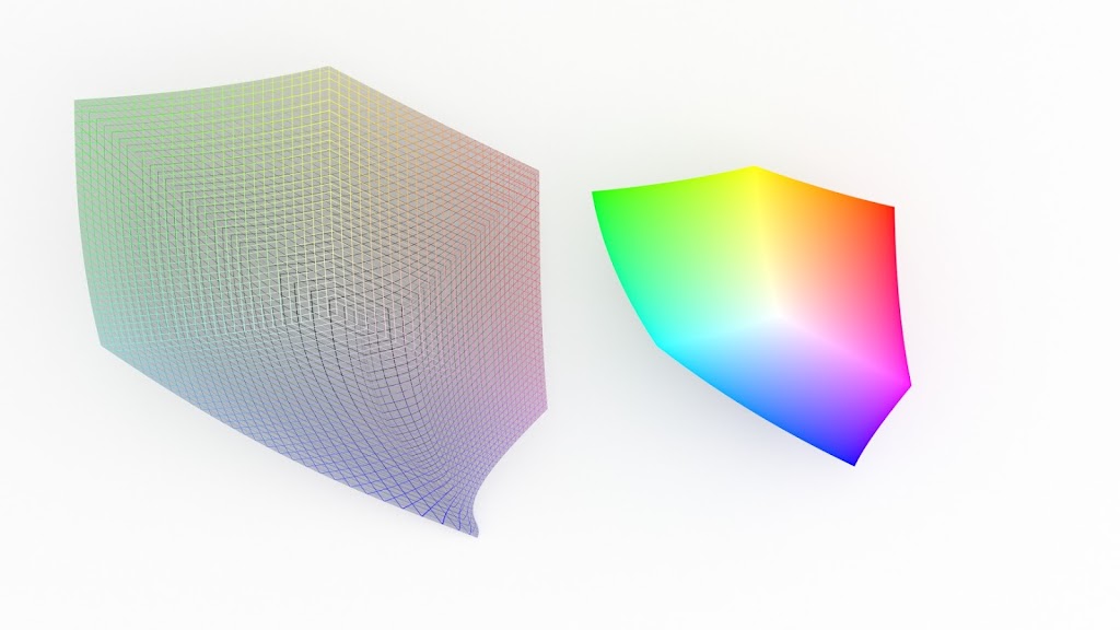
Although RGB coordinates are very intuitive for photoshop users, for various reasons they are not the best way to compare different spaces. Converting the RGB values to CIELAB space is almost always a better choice because CIELAB is not device dependent and is closer to being perceptually uniform. It's still a three dimensional space, but instead of R,G, and B, the space is defined by L, a, and b coordinates. By converting colors to CIELAB you can meaningfully compare different colorspaces—you can plot the gamut of your monitor against the gamut of your printer, or plot colors of a photograph against a working space to see which colors will fall out of gamut in a color conversion. Not quite as useful, but still common practice is calculating the volume of an entire color space. This gives you a single number representing the size of a color space's gamut. Because the conversion to CIELAB space is not linear, calculating the volume of this space is a little tricky, but luckily there are applications and websites to help the color nerd along in his quest for impractical bits of trivia. But here's a small problem: the various applications and websites report different numbers even for well-defined and relatively simple color spaces such as the common working spaces. For instance:

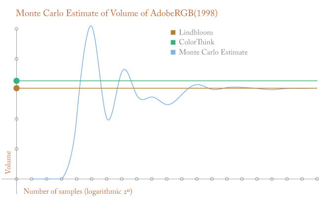
AdobeRGB(1998) Gamut Volume
Bruce Lindbloom: 1,208,631
ColorThink Pro: 1,306,820

This is a fairly large discrepancy for something as well-defined as AdobeRGB(1998). I have no idea how Lindbloom or ColorThink arrived at their numbers, but both are well respected so I've always accepted that this is just hard to do. Honestly, I have no idea how to calculate the volume of AdobeRGB analytically. But there are a lot of problems, especially in the physical sciences, that are difficult to solve analytically, that can nevertheless be estimated to arbitrary precision using other methods. One method is called the Monte Carlo method. It is a little quirky and counterintuitive because it uses random numbers to arrive at a non-random estimate, but it is well-studied and works predictably.

Monte Carlo Method

Imagine a complicated shape whose area you want to determine. One way to estimate the area is to confine the shape within another shape with a known area. For instance, draw a square that completely encloses the shape. The area of the square is easy to calculate and provides an upper limit of the area of the original shape—it must be a percentage of the area of the square that encloses it. The Monte Carlo method will estimate that percentage. You begin by picking random points—and it's important that they are truly random—within the square and taking note of how many also fall within the complicated shape.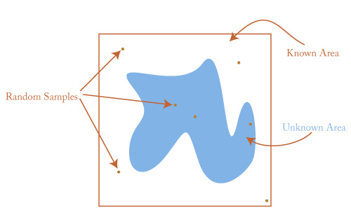

Since the points are randomly distributed, the odds of a point falling within the shape are the same as the proportion of the unknown area to the known area. If you pick 1000 random points and 400 fall within the unknown area, you can make a decent guess that it is about 40 percent the size of the known area. If the square is 100 square units, the unknown area should be around 40 square units. The more points you sample, the more accurate your estimate will be. A nice feature of the Monte Carlo method is that the error is a predictable function of the number of points: 1 over the square root of the number of samples. It's easy to see how this works with a simple two-dimensional shape, but the Monte Carlo method has a killer feature—it doesn't care how many dimensions you are working with. Three dimension? Eighty dimensions? It still works. This is very handy in the physical sciences where problems involving many degrees of freedom are common. Since the problem of computing color gamut volumes only needs three dimensions, this method should work, but let's test it on a known volume first to make sure.

Computing the volume of a sphere

Take a sphere with a radius of 0.5. Its volume is easy to calculate analytically because we know the formula. For a sphere with a radius of 0.5, the volume is about .5236. But let's pretend we don't know that. To use the Monte Carlo method, imagine a cube that completely encloses the sphere. A cube with sides of 1 and hence an volume of 1 cubic unit (we picked a .5 radius for a reason) will perfectly enclose the sphere—we know the volume of the sphere is less than 1 because it fits perfectly inside the cube but does not fill it.

To estimate the ratio of the sphere's volume to the cube's volume pick random points within the cube and calculate whether the points also fall within the sphere. If you place the center of the sphere at the origin this easy to calculate. Since the cube is also centered at the origin, the random points will all have coordinates the between -0.5 and 0.5. Any point with a distance greater than 0.5 from the origin will fall outside the sphere— it will be in the corners of the cube that the sphere doesn't reach.

For example, five random points:
(0.29572273, -0.19648981, 0.33975443) inside sphere
(-0.34014496, 0.05262803, 0.1005302) inside sphere
( 0.28505572, 0.15252012, -0.39578995) outside sphere
( 0.38792913, 0.33801827, 0.4455285 ) outside sphere
( 0.0226319, -0.16996851, -0.49685406) outside sphere

Out of five samples, two, or 40%, fell inside the sphere and we estimate the sphere's volume at 40% of the cube's known volume of 1, or 0.4 cubit units. Not bad compared to the known volume of the sphere, 0.5236, but not particularly good. Since we are using a computer, we don't have to settle for this—we can take a lot more than five samples. We can take thousands or millions. Here is a graph of our estimate (the blue line) compared to the actual volume (orange line) as we take more and more samples.

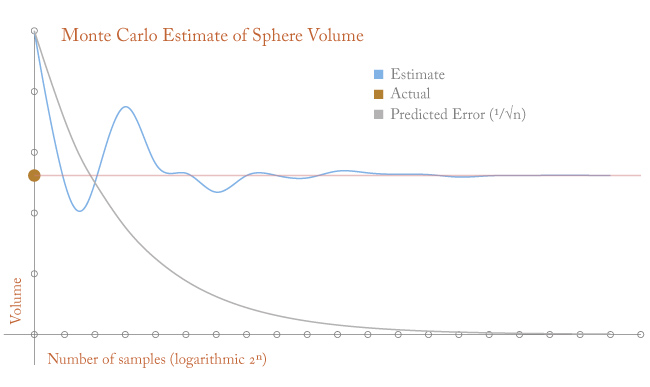
As the number of samples increases our estimate converges on the correct value. With enough patience and computer power we can estimate the volume of the sphere to arbitrary precision. Pretty cool for such a simple idea.

Color Gamuts

The problem of estimating gamut volume is only a little more complicated than the sphere. Here's what we need:

1. The color space in question. We'll use AdobeRGB(1998)
2. An easily-calculated volume that encloses the color space. We'll use a volume defined in CIELAB with L between 0 and 100 and a & b between -128 and 128. This is a much bigger volume than we need, but we can be certain that AdobeRGB fits easily within it.
3. A way to determine if the random values within the know volume also fall within the unknown space.

Point three is the only part that's different from the sphere problem and it's not difficult. We will be picking random LAB values. To see if a point falls within the color space we are testing, we simply convert the LAB values to AdobeRGB. After the conversion, coordinates with values less than zero (you can't have negative RGB values) or more than 100% of a primary are out of gamut and by definition are not within the volume. Here's an example:

A randomly selected LAB value:
(63.7967144778, -10.2849561262, 24.0205449766)
Translate to AdobeRGB space:
(150.186414985, 157.890421952, 112.784324036)
All RGB value are greater than 0 and less than 255. It's a nice, light olive green that falls easily within AdobeRGB

The Next Point:
(31.6022297666, 28.6536083494, 91.1539008272)
Translate to AdobeRGB:
[110.22529566, 55.7252026698, -54.164476]
You can't have a negative blue value, it's way out of the AdobeRGB gamut.

So now we simply repeat this a few million times, just like the sphere example, and keep track of how many are in gamut compared to the total number sampled. The ratio between the total number of samples and those that are within the AdobeRGB gamut should be the same as the ratio between the known LAB volume and the unknown AdobeRGB space. Here's a graph of how the estimate begins to converge as the number of samples increases.

Conclusion

After a little over eight million samples this method zeroes in on Bruce Lindbloom's calculation. At my next cocktail party I will be able to confidently drop the AdobeRGB(1998) gamut volume of 1,208,631 into casual conversation. Sorry ColorThink.